Materials and Methods

This chapter describes the methodology that developed this work and the tools used to achieve the results. This work proposes a method for autonomous 2D image navigation in a 3D model of the hand, based on anatomical landmarks. The agent is trained using reinforcement learning to navigate through the labeled volume with the goal of reaching the optimal standard view of the carpal tunnel. The reward function is based on the presence of anatomical landmarks, such as bones, tendons, and the ulnar artery, and their relative position, tuned on the anatomical description of the optimal slice.

The methodology is summarized in Fig. 14. The first step of the work is the segmentation of the MRI volumes, which consists of labeling the anatomical structures upon which the reward is based. Then, a method for arbitrary slicing is implemented to navigate through the 3D volume by viewing different image planes of the hand. Features extraction is performed by clustering the segmented regions into anatomical landmarks that can be used to calculate the reward function. The reward function is based on the number of clusters detected for each tissue, which is compared to the desired anatomical description of the optimal view of the carpal tunnel. The navigation can be formulated as a search and optimization problem. The agent is trained using reinforcement learning in a simulation environment modeled on the Gymnasium API.

Fig. 14 Methodology for autonomous 2D image navigation in a 3D model of the hand. The agent is trained using reinforcement learning to navigate through the labeled volume to reach the optimal standard view of the carpal tunnel.

MRI Data-set

Availability of data and data quality is often a problem when training a machine learning agent, even more so in the medical field, where collecting patient data is time-consuming and expensive. This work uses a freely available data-set [1] of MRI scans of the hand collected by Wang, Matcuk, and Barbic at the University of Southern California [8].

The data set contains 48 MRI scans of the hand, collected from 4 subjects each scanned 12 times in different poses. The poses are the same for all subjects. The files are in the NIfTI format, a standard format for medical imaging data. Moreover, the same data set has already been partially segmented and made publicly available [2] in [9], for studies related to virtual and augmented reality in healthcare. In the scope of this study, the research group had segmented the bones of the hand, to achieve a more realistic bio-mechanics analysis. Also, these files are in the standard NIfTI format.

For the algorithm to work, all the anatomical features upon which the reward is based must be fully labeled along the volumes. These are bones, the flexor tendons of the fingers, and the ulnar artery. The labelmaps of the hand bones were the starting point for segmenting the MRI volumes. The fully segmented labelmap volumes were then used to generate the environment in which the agent is trained.

Segmentation

Segmentation consists of defining the contours of specific structures in the image. In the field of medical imaging, segmentation is a common task, used for multiple purposes, such as diagnosis, pre-operative planning, or use of computer-aided surgery. It requires a good anatomical knowledge of the region of interest and a good understanding of the imaging modality used to acquire the images.

To recognize certain anatomical structures, it is often not sufficient to look at one image only. It is necessary to analyze the relations between structures in sequential slices, to understand how they develop in the body. Moreover, it is important to visualize the same structure in different orientations, to comprehend its 3D shape.

Segmentation Software

Labeling was performed using the ImFusion Suite software [3] [10], which is a medical image analysis tool that allows the segmentation of anatomical structures in 3D volumes. The software provides simultaneous visualization of the volumes in four quadrants: three display the orthogonal axial 2D projections or slices of the volume, while one presents the fully rendered 3D volume. The orthogonal projections will be defined as frontal, for the top, longitudinal, for the side, and axial, for the transversal view. Users can scroll through the axial slices and adjust their orientation to view sections of the hand from various angles.

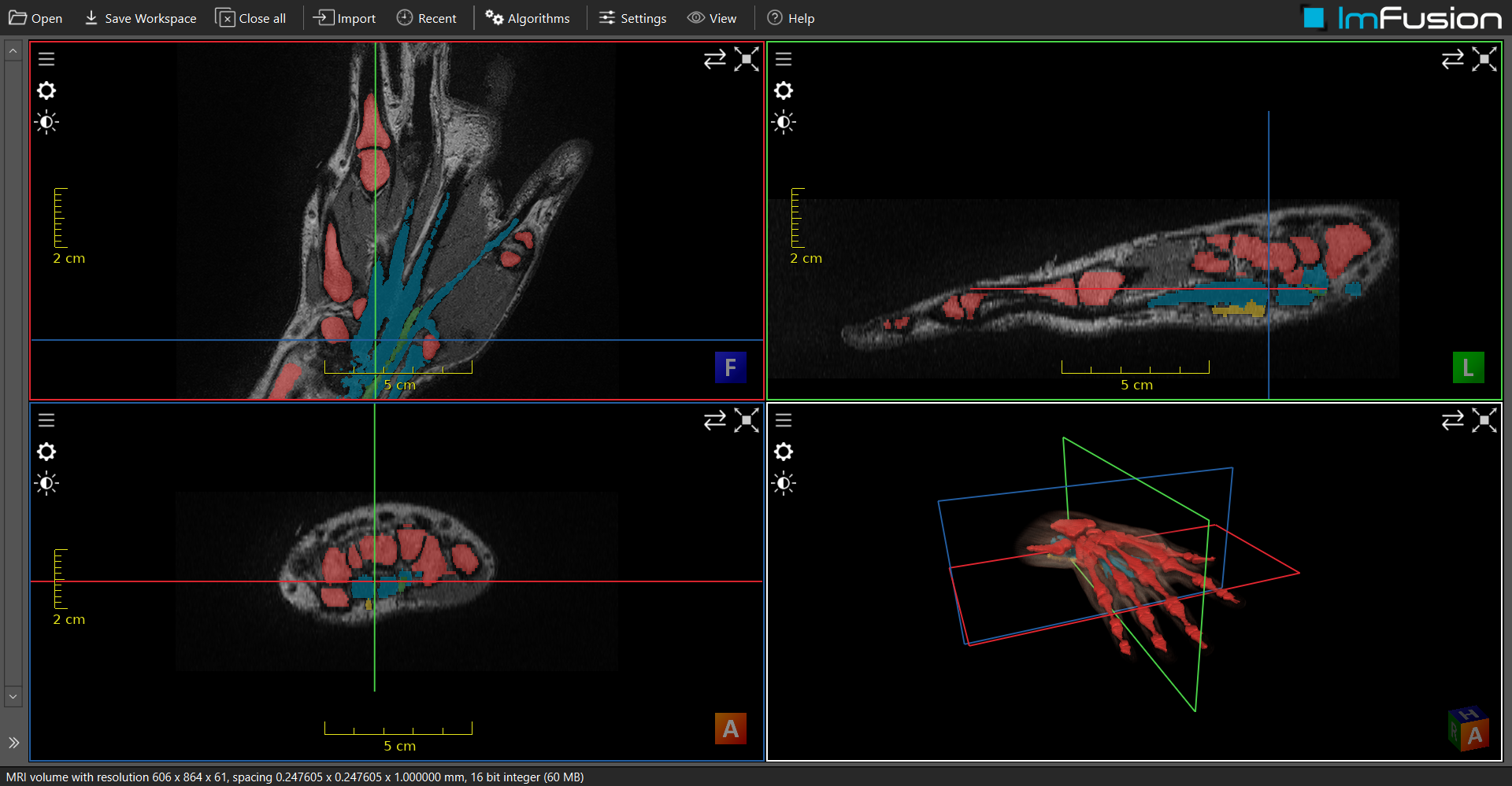
Fig. 15 Superposed fully segmented labelmap and MRI volumes of a hand in ImFusion Suite software interface [10].

The segmentation toolbox offers a variety of tools to segment the images. The most important ones are the brush and the eraser, with which the user can draw or delete the contours of the structures. When using the brush on a 2D projection, the corresponding region is also shown and segmented in the corresponding points of the other two projections. The brush size is defined as the diameter of a 3D sphere and can be adjusted in size (mm).

Another important parameter of the brush is its adaptiveness, which adjusts the size and contour of the brush. Adaptiveness accounts for the intensities of the image voxels and labels only those with similar intensities to the ones in the center of the brush. Higher adaptiveness means that the brush will be more selective and conservative in labeling.

The segmentation results are superposed to the medical images, and a 3D mesh can be previewed simultaneously over the 3D render of the original volume. Once the process is complete, the labelmaps can be exported in the NIfTI format.

Labeling Process

As mentioned before, the navigation system is based on the presence of anatomical labels, in particular the bones of the hand and the wrist, the flexor tendons of the fingers and the ulnar artery. The starting point for segmentation was the labelmaps of the bones of the hand, which were already available. The rest had to be segmented from the MRI volumes. To recognize the anatomical structures in the MRI images, an annotated data set of wrist MRI images from Muskoloskeletal MRI [4] [11] was used as a reference. One specifically important slice was that of the carpal tunnel at the pisiform-scaphoid height shown in Fig. 16.

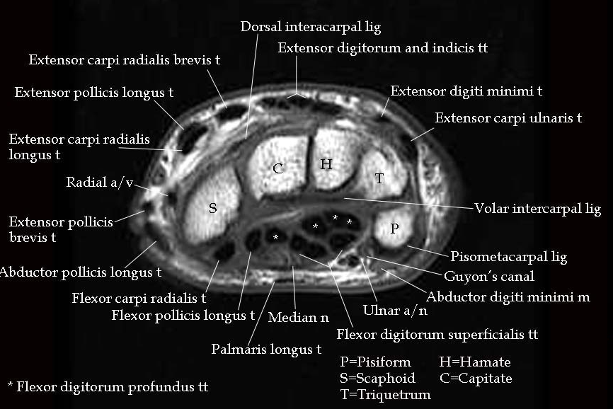
Fig. 16 Transversal view of the carpal tunnel at the pisiform-scaphoid level used as a reference in the segmentation process. Figure from [11].

The raw MRI data and the labelmaps of the bones were loaded into the software and superposed to each other. The orientation of both volumes was aligned to correspond, and their origins were set to zero.

The main difficulty in segmenting the MRI volumes was the low resolution of the images compared to the reference annotated data set. These were often blurry and the separation between the tissues was not always clear.

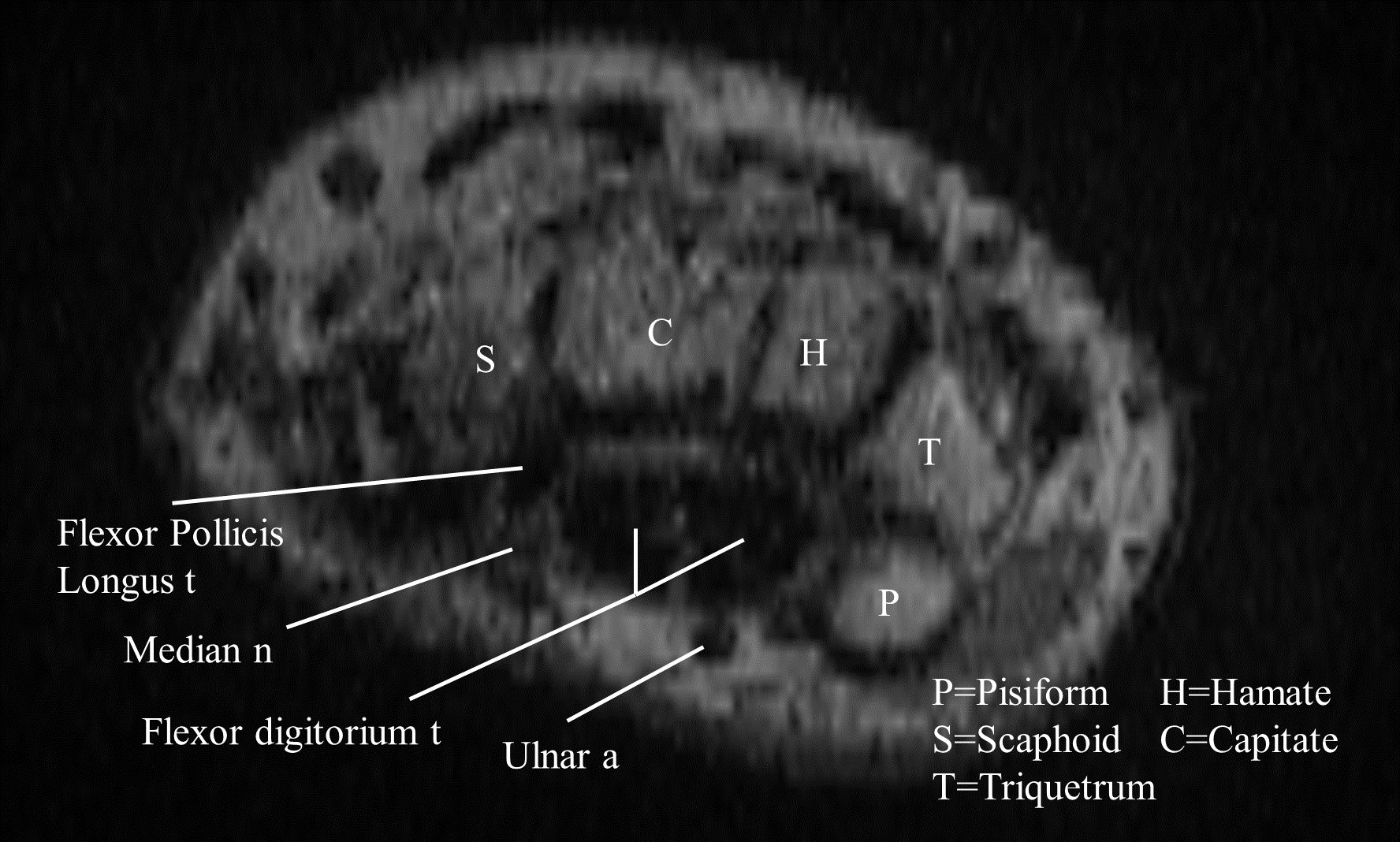
Fig. 17 Transversal view of the carpal tunnel at the pisiform-scaphoid level from one of the data set’s volumes.

The initial step involved segmenting the radial and ulnar bones of the wrist, which were not included in the segmentation by [9]. It was essential to ensure that the segmentation was consistent and without gaps, as any inconsistencies could mislead the clustering algorithm used in later stages. Segmenting the bones was relatively straightforward due to their high contrast with the surrounding tissues.

Next, the flexor tendons of the fingers were segmented. Tendons are easily identifiable in MRI images as large dark structures. The flexor tendons extend from the wrist to the fingers and are also well-recognizable in the forearm. The optimal method for segmenting them was to use a relatively large brush size with high adaptiveness. The brush’s shape adjusts well to the tendons due to the significant intensity difference from the other tissues. The tendons are clearly visible in the axial view of the forearm and wrist, but it is more practical to continue the segmentation in the frontal view, where they can be traced along the palm. The longitudinal view is most effective for segmenting the tendons in the fingers after adjusting the orientation to be parallel to each finger.

Subsequently, the ulnar artery was segmented. Like all vessels, the artery is recognizable by its elongated shape and dark appearance, similar to tendons, but it is much smaller and runs alone. It is easily localized in the axial view of the carpal tunnel, and once segmented in that region, it can be identified in the frontal view of the forearm, provided the axis is well-aligned with the forearm. A small brush size with high adaptiveness was used for this segmentation.

Finally, the median nerve was segmented. Although the nerve is not a reward feature in the navigation algorithm, it was labeled to achieve a complete segmentation of the carpal tunnel. The nerve is the most challenging structure to recognize due to its inconsistent size and shape and low contrast with surrounding tissues. For this reason, it was not selected as a reward feature. It is best recognized in the axial view of the carpal tunnel, owing to its spatial relationship with the tendons running through the tunnel. It can then be traced in the longitudinal view of the forearm, as it runs just beneath the flexor digitorum profundus tendons.

Volume Processing

Standard planes are important in medical imaging because they provide a method to compare biometric measurements of anatomical regions. To get an optimal view of a specific standard plane, it is necessary to navigate through the images viewing different orientations. MRI volumes are 3D images composed of a series of 2D images, or slices, taken at regular intervals along three axes. Often, the set of possible views is constrained to the orientation at which the image acquisition has been performed. However, the ability to arbitrarily navigate the images with any orientation is crucial for medical imaging analysis.

Computer systems for image processing allow to recreate a 3D volume from the stack of 2D images by interpolating the intensities of the voxels between the slices. This allows one to visualize the volume from any angle and to slice it in any direction, which has become an indispensable tool for extracting information from medical images [12] . ImFusion Suite software allows to view the volume in any orientation in their 3D render, which was essential in the labeling process, but to the best of our knowledge it does not offer an open-source and documented integration for Python scripts.

As an alternative, image processing was performed using the SimpleITK [5] library [13][14]. SimpleITK is a simplified layer built on top of the Insight Segmentation and Registration Toolkit (ITK), a powerful open-source software system for image analysis. The fundamental elements of SimpleITK are images and spatial transformations. An image is defined by a set of structured points occupying a physical space, which is determined by the image origin, spacing, size, and direction of the axes corresponding to the matrix columns. Transformations are available for both 2D and 3D spaces and are defined by a matrix \(A\), a center of rotation \(c\), and a translation vector \(t\):

\[T(x) = A \cdot (x - c) + c + t.\]

These characteristics—spacing, size, origin, and orientation—are all stored within the NIfTI file format, a widely used format in medical imaging for storing MRI data. The NIfTI format encapsulates this crucial metadata, ensuring that the spatial relationships within the image are preserved. This information is essential for accurate image analysis and processing, as it allows the software to interpret the physical dimensions and alignment of the scanned volume accurately. By preserving these details, SimpleITK can effectively manage and manipulate the images, maintaining their spatial integrity throughout various transformations and processing steps. The dataset loading process was standardized using a registry and a custom class called ImageVolume, which exploits the properties of NIfTI files and the functionalities provided by SimpleITK.

Resolution Normalization

The resolution of an MRI image is determined by the number of images acquired to scan the volume and is defined by a property called spacing. Spacing represents the physical distance between the image slices taken along each axis, typically measured in millimeters. This spacing also defines the distance between the centers of voxels within the image, where a voxel is the 3D equivalent of a pixel in two-dimensional images. Since spacing is often not isotropic, the distance between voxels can vary across the three directions. By multiplying the pixel spacing by the number of voxels along each axis, one can determine the physical dimensions of the image.

\[\text{Physical size} = \text{Spacing} \times \text{Size}.\]

The resolution of the images in the dataset is not consistent, meaning that their size and spacing vary across the volumes. This inconsistency can affect the clustering algorithm, as the distance between the voxels is not uniform. To address this issue, the images can be normalized to the maximum resolution of the dataset when loading it. This normalization process involves resampling the images to a common resolution, interpolating the voxel values to fit the new size. Since the labelmaps volumes are integer values representing the labels of the segmented structures, the interpolation is performed using the nearest neighbor method, which assigns the value of the nearest voxel to the new voxel, so to maintain the integrity of the labels.

Arbitrary volume slicing

To visualize arbitrary slices of the 3D volume, the function get_volume_slice of the ImageVolume class utilizes a transformation matrix that defines the plane of the slice in the reference frame of the volume. This matrix is defined by the rotation and translation parameters that determine the orientation and position of the slice within the volume. The SimpleITK library provides a convenient way to achieve this using the Euler3DTransform class, which allows for easy setting of rotation and translation. All the volumes have a consistent reference frame orientation, with the X-axis following the direction of the width of the palm, the Y-axis in the direction of the length, pointing towards the fingers, and the Z-axis traversing the depth of the hand, as visualized in Fig. 18.

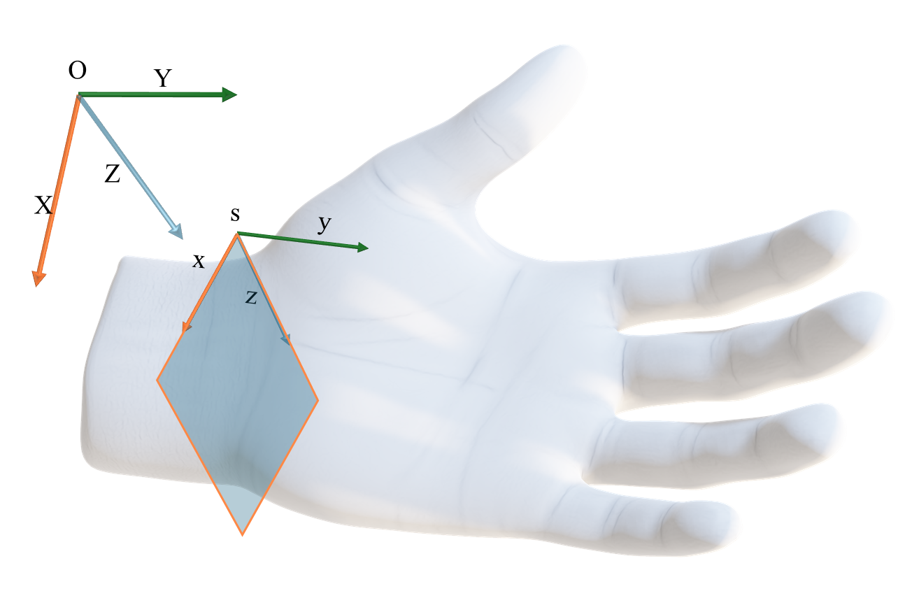
Fig. 18 The reference frame of the MRI volumes, \(O\). The X-axis follows the direction of the width of the palm, the Y-axis in the direction of the length, pointing towards the fingers, and the Z-axis traversing the depth of the hand. An arbitrary slice of the volume is determined by the transformation \(T_{O:s}\) from the origin of the volume \(O\) to the coordinates of the image plane \(s\).

A slice is defined by the transformation \(T_{O:s}\) from the origin \(O\) of the volume to the coordinates of the image plane \(s\). The transformation matrix is composed of a rotation matrix \(R\) and a translation vector \(t\), which are applied to the origin of the volume \(O\):

\[T_{O:s}(x) = R_{O:s} \cdot (x - O) + O + t_{O:s},\]

The slicing function considers only two rotations: around the Z-axis and the X-axis. Rotation around the Z-axis aligns the slice parallel to the wrist, which is essential for obtaining a parallel view of the desired anatomical structure. Rotation around the X-axis adjusts the angulation of the slices. Notably, rotation around the Y-axis is not applied because it would not change the viewing plane, but rather the orientation of the slice within the plane.

Translation is applied along the X and Y axes to position the slice appropriately. The X-axis translation moves the slice transversely, while the Y-axis translation moves it longitudinally. There is no translation along the Z-axis, as this would dig into the depth of the volume.

The image is then sampled from the volume using the SimpleITK resampling method, which requires the transformation matrix \(T_{O:s}\), the size of the slice, and the interpolation method, which is set to the nearest neighbor to preserve the integrity of the labels.

Optimal Slice Labeling

For each volume, the optimal slice for visualizing the carpal tunnel has been pre-labeled by saving the corresponding transformation parameters as attributes of the ImageVolume class. This labeling is crucial for both validation and dimensionality reduction in the analysis. Specifically, to ensure that the clustering and reward functions accurately identify the optimal plane of the carpal tunnel, a test function was implemented. This function verifies that the score for the optimal slice in each volume remains below a predefined threshold, \(\delta = 0.05\), ensuring high precision in the selection process.

Dimensionality reduction is essential for simplifying the navigation problem by reducing the agent’s exploration space. By fixing certain transformation parameters to their optimal values, the degrees of freedom can be restricted focusing on a smaller subset of variables. For example, during a linear sweep, the parameters for x- and z-rotation, as well as x-translation, are set to their optimal values, leaving only y-translation to vary. This approach significantly reduces the complexity of the problem, allowing for more efficient exploration of the state space and a simpler validation of the proposed methods.

Random Volume Transformation for data Augmentation

To enhance the robustness of the model and expand the dataset, small random transformations are applied to the 3D volumes, effectively generating new training samples from existing data. These transformations are deliberately small but sufficient to alter the location of the optimal slice, providing the necessary variability for effective data augmentation.

The TransformedVolume class is designed to handle these transformations. It extends the base ImageVolume by applying a transformation to the volume including rotation and translation. The random transformations are sampled from a predefined range within small bounds — a rotation range of 10 degrees and a translation range of 10 mm — ensuring that the transformations remain small.

The transformations change the position of the 3D image within the original coordinate frame, hence the origin \(O\) stays unvaried, but the image has a new orientation that can be defined with a new coordinate frame. Let the origin of the original volume be defined as \(O_o\) and the origin of the transformed volume as \(O_t\). The transformation matrix \(T_{O_o:O_t}\) is defined as:

\[\begin{split}\begin{aligned} & T_{O_o:O_t}(x) = R_{O_o:O_t} \cdot (x - O_o) + O_o + t_{O_o:O_t}, \\ \text{and} \; & V_{O_t} = T_{O_o:O_t}(V_{O_o}), \end{aligned}\end{split}\]

where \(V_{O_o}\) is the image volume in the original coordinate frame and \(V_{O_t}\) is the image volume in the transformed coordinate frame.

The rotations are performed around the Z-axis and X-axis, consistent with the volume’s reference frame. By rotating around these axes, the view of the volume can be slightly shifted. Translations are applied along the X-axis and Y-axis, moving the image volume transversely and longitudinally in the coordinate frame. These small translations are sufficient to shift the location of the optimal slice, thereby introducing a variety of new slice positions for the model to learn from.

These transformations are implemented using the Euler3DTransform class from SimpleITK. The resampling process, similar to the one used for arbitrary slicing, applies this matrix to the volume, generating a new, transformed volume. Nearest-neighbor interpolation is used during resampling to preserve label integrity. After transformation, the volume is treated as a new ImageVolume, but its optimal plane is recalculated to reflect the changes in orientation and position. The transform_action method allows to transform any transformation defined in the original coordinate frame with origin \(O_o\) to the new one defined in \(O_t\), by applying the inverse of the transformation matrix \(T_{O_o:O_t}(x)\) to the transformation to reach the optimal plane \(T_{O_o:s}\):

\[\begin{split}\begin{aligned} & \begin{aligned} T_{O_t:s} & = T_{O_t:O_o} \cdot T_{O_o:s} \\ & = (T_{O_o:O_t})^{-1} \cdot T_{O_o:s}, \end{aligned} \\ & T_{O_t:s}(x) = R_{O_t:s} \cdot (x - O_t) + O_t + t_{O_t:s}, \end{aligned}\end{split}\]

and \(T_{O_o:s}\) and \(T_{O_t:s}\) are the transformations from the origin of the volume to the coordinates of the image plane in the original and transformed coordinate frames, respectively.

By introducing these small, random transformations, the variability within the dataset can be increased. This variability is key to improving the model’s ability to generalize, as it learns to navigate to the optimal plane across a range of slightly different orientations and positions, ultimately enhancing its performance in real-world clinical scenarios.

Anatomical Reward Function

The goal of the agent is to navigate through the labelmaps of the MRI volumes and find the optimal standard view of the carpal tunnel. State of the art methods for anatomical navigation to a standard plane are based on the use of a reward function that scores the distance from the current plane position to the target plane, calculating the Euclidean distance between the two points and the difference in orientation. With this reward configuration, the agent will not get any feedback outside of the training environment, and the navigation will then be based on the features extracted from the real-time images by the CNN. This approach has the limitation of a black box model since it is not predictable to know how the agent will behave in a real environment, and whether it will be able to generalize the learned features to new data.

In this work, the reward function is based on the anatomical landmarks of the images, in a similar way to how medical professionals would navigate towards a standard plane. The landmarks for carpal tunnel navigation were selected to follow medical protocols, such as those described in [15][16][17] . The anatomy of the soft tissues is generally very prone to inter-patient variations in size, shape, and position, and it changes with movement and muscle activation. Bones, however, are an invariant landmark that offers a more stable reference for localizing the other tissues. Nevertheless, the flexor tendons of the fingers in the carpal tunnel are also a good landmark. They are grouped in the middle of the wrist, in a way that makes it easy to recognize the tendons cluster. Lastly, the ulnar artery offers another natural landmark, since it is easy to recognize its circular black shape and runs right above the tendons.

Bones, tendons, and the ulnar artery are the features that will be used to calculate the reward function. In particular, the absence of these landmarks will be hardly penalized. At the same time, their presence, the amount of clusters detected for each tissue, and the relative position of the clusters to each other will be rewarded. The score of each slice is defined as a negative loss function bounded between \([-1, 0]\), where \(0\) is the optimal score for a slice that corresponds to the description of the standard plane. The loss function is defined as the sum of three components, which are then normalized:

\[loss = -\frac{1}{3}(clusters\_number + missing\_landmarks + relative\_position). \label{eq:reward}\]

The first term evaluates the number of landmarks detected for each tissue. The optimal number of landmarks is based on the anatomical description of the optimal slice. For instance, the ulnar artery is a single landmark, thus only one cluster is expected. The number of bones depends on the view of the carpal tunnel, varying from five at the level of the Scaphoid-Pisiform to four at the level of the Hamate-Hook. The choice of four as a reference number showed better results throughout the dataset, and was then set as the expected number of clusters. Bone clusters are well-defined because they are easy to segment. However, segmenting tendons is more challenging, particularly in the carpal tunnel region where they are grouped in a small area. The dataset resolution also did not allow for a clear separation of the tendons, as shown in Fig. 17. Therefore, the number of tendon clusters is not consistent with the anatomy of the CT, which would expect eight separate landmarks, as visible in Fig. 16. Nonetheless, the number of tendon clusters detected at the carpal tunnel level turned out to be consistent across the dataset, and it was set to three. The loss related to the number of clusters is defined as the difference between the expected and detected number of clusters for each tissue, normalized by the total number of clusters:

\[clusters\_number = \frac{1}{8}(n_{bones} + n_{tendons} + n_{artery}), \label{eq:clusters}\]

where \(n_{bones}\), \(n_{tendons}\) and \(n_{artery}\) are the number of clusters detected for each tissue in the current slice. The decision to normalize the total number of landmarks, rather than normalizing for each tissue individually, is motivated by the desire to give equal importance to each independent landmark.

The second term imposes an additional penalty for the complete absence of any tissue in the slice. While the first term does account for this, it is important to more heavily penalize the total absence of a landmark compared to merely detecting an incorrect number of clusters. This adjustment also ensures a balanced representation of the ulnar artery, which forms a single cluster, relative to the bones and tendons that have multiple clusters and therefore exert a greater influence when compared with the expected number of clusters. As a result, it is essential that all three tissues are present and detectable within the optimal region. This penalty is defined as:

\[missing\_landmarks = \frac{1}{3}(missing\_bones + missing\_tendons + missing\_artery), \label{eq:missing}\]

where the missing features are binary values, either \(0\) or \(1\), indicating the absence or presence of the tissue in the slice, respectively.

The last term evaluates the relative position of the clusters to each other. In detail, it checks that the bones are located at the bottom of the slice, the tendons in the middle, and the ulnar artery at the top. The relative position is calculated by taking the mean of the coordinates of the centroids of the clusters for each tissue and comparing their relative position. The centroid of the tendons’ clusters is expected to be between the centroid of the bones and the artery. The loss related to the relative position is either \(0\) if the relative position is correct or \(1\) if it is not:

\[\begin{split}\text{relative\_position} = \begin{cases} 0 & \text{if } \mu_{y:\text{bones}} < \mu_{y:\text{tendons}} < \mu_{y:\text{artery}} \text{ or } \mu_{y:\text{artery}} < \mu_{y:\text{tendons}} < \mu_{y:\text{bones}} \\ 1 & \text{otherwise} \end{cases}, \label{eq:relative}\end{split}\]

where \(\mu_{bones}\), \(\mu_{tendons}\), and \(\mu_{artery}\) are the mean coordinates of the centroids of the clusters for each tissue in the current slice.

Clustering for Landmark Detection

The clustering algorithm is essential to detect and group the segmented regions into landmarks. In particular, it is necessary to determine the number of clusters of each landmark type present in the images. While segmentation identifies which pixels belong to which type of tissue, clustering groups these segmented pixels into distinct anatomical landmarks. The outcome of the clustering process directly influences the reward function used in our algorithm.

Centrosymmetric Mask Clustering

Initially, clustering was implemented using the label function from the ndimage module in SciPy [6], which adopts a centrosymmetric binary mask to identify neighboring elements of the same value, which can be defined as:

\[\begin{split}\begin{bmatrix} 0 & 1 & 0 \\ 1 & 1 & 1 \\ 0 & 1 & 0 \\ \end{bmatrix}.\end{split}\]

For a 2-dimensional image or array with some features, the label function identifies the connected components of the features in the image. To find the clusters of each tissue, a binary mask was created for each tissue type, which would set the pixels corresponding to the segmented regions to 1 and the rest to 0. The label function then groups the connected pixels into clusters, which are assigned a unique integer label. The number of clusters is determined by the number of unique labels present in the resulting array.

Although straightforward, this method has notable limitations. If two groups of features have connected elements, the label approach from ndimage counts them as a single cluster, making it impossible to separate closely situated clusters. Additionally, there is no provision to set a minimum standard size for clusters, which means that small outliers from incorrect segmentation cannot be excluded. The issue is evident in Fig. 19, where two different bones are clustered together due to their proximity, and many smaller clusters are detected as well.

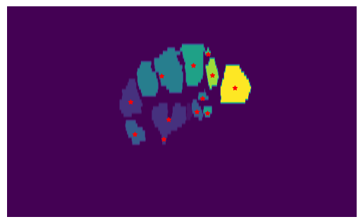
Fig. 19 Clustered slice of a labeled MRI volume using the ndimage label function. The different colors represent the different clusters detected by the algorithm. The center of each cluster is depicted by a red star. It is visible how two different bones are clustered together due to their close proximity, and many smaller clusters are detected as singular landmarks instead of being grouped together or assigned to noise.

Example

Consider the following 2D array:

\[\begin{split}\begin{bmatrix} 0 & 0 & 1 & 1 & 0 \\ 0 & 0 & 1 & 1 & 0 \\ 1 & 1 & 0 & 0 & 0 \\ 0 & 0 & 1 & 1 & 0 \\ 0 & 0 & 1 & 0 & 0 \\ \end{bmatrix}.\end{split}\]

The label function would group the connected pixels into clusters, yielding as a result the labeled array

\[\begin{split}\begin{bmatrix} 0 & 0 & 1 & 1 & 0 \\ 0 & 0 & 1 & 1 & 0 \\ 2 & 2 & 0 & 0 & 0 \\ 0 & 0 & 3 & 3 & 0 \\ 0 & 0 & 3 & 0 & 0 \\ \end{bmatrix},\end{split}\]

and the number of clusters, which in this case is 3.

First Clustering and Reward Validation on Suboptimal Linear Sweep

In order to validate the use of an anatomical reward function based on the clustering results, an exhaustive search was performed along the axial slices of one labelmap volume. The goal was to find the optimal slice that maximizes the reward function, demonstrating that the reward function can effectively guide the agent to a globally optimal region.

The first fully segmented labelmap volume was used for the validation. Unfortunately, the standard view of the carpal tunnel was not visible on the axial slices of MRI scan, since this had been acquired in a different orientation. Since no function to perform arbitrary slicing had been implemented yet, it was impossible to get a view of the carpal tunnel in the standard plane. Therefore, the reward function was tuned on the anatomical description of a suboptimal view of the carpal tunnel, which was visible in the axial slices. In particular, the number of landmarks was set to 7 bones, 5 tendons and 1 ulnar artery.

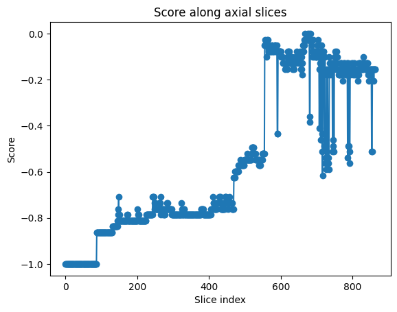
Fig. 20 Reward values for each axial slice of the volume. In proximity to the carpal tunnel, the anatomical score is 0, indicating the optimal correspondence to the anatomical description.

The exhaustive search was performed by sweeping through the axial slices of the volume, performing clustering, and calculating the reward function for each slice. The results shown in Fig. 20 demonstrate the presence of a global optimum, which corresponds to the described sub-optimal view of the carpal tunnel.

DBSCAN

To overcome the limitations of the ndimage approach, the DBSCAN (Density-Based Spatial Clustering of Applications with Noise) algorithm was adopted [18][19] , implemented using sklearn [7]. DBSCAN offers several advantages over the initial method. First, DBSCAN identifies clusters based on the density of data points, enabling it to distinguish clusters even if they are close together, provided there is an area with a lower density of points separating them. Furthermore, DBSCAN can identify and discard noise or outliers, which is particularly useful for eliminating small erroneous segmentations.

DBSCAN works by defining two parameters: \(\epsilon\), which sets the maximum distance between two samples for them to be considered in the same neighborhood, and \(min\_samples\), which sets the minimum number of samples in a neighborhood for a point to be considered a core point. The algorithm then groups the points into clusters based on these parameters. The result is a set of clusters, each assigned a unique integer label. Points that are not part of any cluster are assigned the label \(-1\), indicating noise.

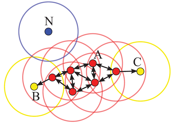
Fig. 21 Illustration of the DBSCAN clustering algorithm, for \(\epsilon\) equal to the radius of the circles and \(min\_samples=4\). The red points are core points and are assigned to the cluster. The yellow points are border points, and the blue point is a noise point. Figure from [19].

The DBSCAN algorithm is illustrated in Fig. 21. Points situated in a dense region with more than \(min\_samples\) neighboring points within a distance of \(\epsilon\) are considered core points and assigned to a cluster. Points that are within \(\epsilon\) of a core point but have fewer than \(min\_samples\) neighbors are considered border points and are assigned to the same cluster as the core point. Points that are not core or border points are considered noise points.

The distance \(\epsilon\) between two points is calculated as the Euclidean distance between their coordinates in the array. The coordinates of these points are determined by the indices of the pixels within the slice. Consequently, the distance is dependent on the image resolution, making it essential to normalize the resolution across all volumes.

DBSCAN Parameters Tuning and Validation

The two parameters \(\epsilon\) and \(min\_samples\) have to be tuned based on the specific characteristics of the landmarks. The optimal values for these parameters were identified by examining the clustering results on the labeled MRI volumes, ensuring consistent detection of clusters across the dataset, as shown in 1.1 tab:dbscan_params. Nevertheless, an optimization process should be implemented to automatically determine the optimal values for these parameters.

Table 3 Optimal values for the DBSCAN parameters \(\epsilon\) and \(min\_samples\) for each tissue type.

Landmark	\(\epsilon\)	\(min\_samples\)	Expected clusters	Suboptimal View
Bones	4.1	46	4	7
Tendons	3	18	3	5
Artery	1.1	4	1	1

The DBSCAN parameters align well with the intuition of an anatomical description. The bones are the largest landmarks and are expected to have the largest clusters, which is reflected in the high \(\epsilon\) and \(min\_samples\) values. The tendons are smaller and might have some low-density regions since they are grouped in a small area, therefore a slightly lower \(\epsilon\) is set and a lower \(min\_samples\) value. The ulnar artery is the smallest landmark and is expected to have the smallest cluster, which is reflected in the lowest \(\epsilon\) and \(min\_samples\) values. The clustering results can be seen in Fig. 21.

Fig. 22 Same slice clustered using centrosymmetric clustering and the DBSCAN algorithm. In the DBSCAN output, the bone clusters are more clearly separated, and the smaller clusters are treated as noise, or integrated into bigger clusters.

The implementation of DBSCAN from the sklearn library significantly enhanced the accuracy and reliability of the clustering process. This improvement is crucial because the reward function in the algorithm depends heavily on the precise detection and grouping of these landmarks. The results of the DBSCAN clustering, illustrated in Fig. 23, show a superior reward function score distribution compared to the ndimage approach. The reward, still adjusted to the same sub-optimal description, achieves a score of 0 for a very well-defined region of the carpal tunnel, with no outliers detected.

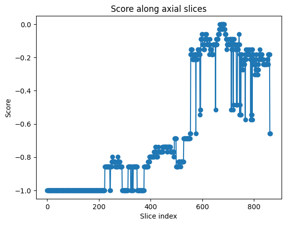
Fig. 23 Reward values for each axial slice of the volume. Shows a more cler optimal region compared to the results of the ndimage clustering.

[1]

https://viterbi-web.usc.edu/ jbarbic/hand-mri-data-set/download.php

[2]

reyuwei/PIANO_mri_data

[3]

https://www.imfusion.com/

[4]

https://freitasrad.net/pages/atlas/Wrist/Wrist.php

[5]

https://simpleitk.org/

[6]

https://docs.scipy.org/doc/scipy/reference/generated/scipy.ndimage.label.html#scipy.ndimage.label

[7]

https://scikit-learn.org/stable/modules/generated/sklearn.cluster.DBSCAN.html

Bibliography

[8]

Bohan Wang, George Matcuk, and Jernej Barbič. Hand mri dataset. 2020.

[9] (1,2)

Yuwei Li, Minye Wu, Yuyao Zhang, Lan Xu, and Jingyi Yu. Piano: a parametric hand bone model from magnetic resonance imaging. In Zhi-Hua Zhou, editor, Proceedings of the Thirtieth International Joint Conference on Artificial Intelligence, IJCAI-21, 816–822. 2021. doi:10.24963/ijcai.2021/113.

[10] (1,2)

ImFusion GmbH. Imfusion. 7/25/2024. URL: https://www.imfusion.com/ (visited on 7/25/2024).

[11] (1,2)

Alex Freitas. Basic-wrist-mri. 2/15/2024. URL: https://freitasrad.net/pages/Basic_MSK_MRI/basic-wrist-mri.php (visited on 2/15/2024).

[12]

Nickolas Papanikolaou and Spyros Karampekios. 3d mri acquisition: technique. In Emanuele Neri, Carlo Bartolozzi, and Davide Caramella, editors, Image Processing in Radiology, Medical Radiology, Diagnostic Imaging, pages 15–26. Springer-Verlag Berlin Heidelberg, Berlin, Heidelberg, 2008. URL: https://link.springer.com/chapter/10.1007/978-3-540-49830-8_2, doi:10.1007/978-3-540-49830-8{\textunderscore }2.

[13]

Bradley C. Lowekamp, David T. Chen, Luis Ibáñez, and Daniel Blezek. The design of simpleitk. Frontiers in neuroinformatics, 7:45, 2013. doi:10.3389/fninf.2013.00045.

[14]

Ziv Yaniv, Bradley C. Lowekamp, Hans J. Johnson, and Richard Beare. Simpleitk image-analysis notebooks: a collaborative environment for education and reproducible research. Journal of digital imaging, 31(3):290–303, 2018. doi:10.1007/s10278-017-0037-8.

[15]

Maureen Wilkinson, Karen Grimmer, and Nicola Massy-Westropp. Ultrasound of the carpal tunnel and median nerve. Journal of Diagnostic Medical Sonography, 17(6):323–328, 2001. doi:10.1177/875647930101700603.

[16]

Sandy C. Takata, Lynn Kysh, Wendy J. Mack, and Shawn C. Roll. Sonographic reference values of median nerve cross-sectional area: a protocol for a systematic review and meta-analysis. Systematic Reviews, 8(1):2, 2019. URL: https://link.springer.com/article/10.1186/s13643-018-0929-9, doi:10.1186/s13643-018-0929-9.

[17]

A. Gervasio, C. Stelitano, P. Bollani, A. Giardini, E. Vanzetti, and M. Ferrari. Carpal tunnel sonography. Journal of Ultrasound, 23(3):337–347, 2020. URL: https://link.springer.com/article/10.1007/s40477-020-00460-z, doi:10.1007/s40477-020-00460-z.

[18]

Martin Ester, Hans-Peter Kriegel, Jörg Sander, Xiaowei Xu, and others. A density-based algorithm for discovering clusters in large spatial databases with noise. In Proceedings of the 2nd International Conference on Knowledge Discovery and Data Mining - 1996, pages 226–231. 1996.

[19] (1,2)

Erich Schubert, Jörg Sander, Martin Ester, Hans Peter Kriegel, and Xiaowei Xu. Dbscan revisited, revisited. ACM Transactions on Database Systems, 42(3):1–21, 2017. doi:10.1145/3068335.