Visualization of MRI Data and Labelmaps#
This notebook contains a tutorial for visualizing medical images, in particular MRI data and Labelmaps. For this purpose we are going to use the library SimpleITK.
Show code cell content
import matplotlib.pyplot as plt
import numpy as np
import SimpleITK as sitk
from armscan_env.config import get_config

config = get_config()
Dataset visualization#
The MRI 3D images are saved as NifTi files under “data/mri” and the label-maps are saved as NifTi files under “data/labelmaps”. To load them, we have implemented a config file that retrieves the path of the files, by just specifying their index. The images are loaded through the SimpleITK library, which allows us to easily manipulate them. In order to visualize the images, we convert them to numpy arrays using the sitk.GetArrayFromImage function. It is important to note that the shape of the data changes when transformed from a SimpleITK image to a numpy array. The original shape of the image is (x, y, z), but the numpy array has the shape (z, y, x). This is important to keep in mind when indexing the array. The origin of the image is also important, as it defines the position of the image in the 3D space.
mri_volume = sitk.ReadImage(config.get_single_mri_path(1))
mri_img = sitk.GetArrayFromImage(mri_volume)
print(f"{mri_volume.GetSize()=}")
print(f"{mri_img.shape=}")
mri_volume.GetSize()=(606, 864, 61)
mri_img.shape=(61, 864, 606)
The size of the array corresponds to the number of images stacked per dimension. The images are stacked along all three dimensions: frontal, longitudinal and transversal. The space between one image and the next is constant for each dimension, and it is stored in the spacing attribute of the SimpleITK image in millimeters. Multiplying the spacing by the size of the array gives the total size of the MRI volume in millimeters.
print(f"{mri_volume.GetSpacing()=}")
size = np.array(mri_volume.GetSize()) * np.array(mri_volume.GetSpacing())
print(f"{size=} mm")
mri_volume.GetSpacing()=(0.24760496616363525, 0.24760496616363525, 1.0)
size=array([150.0486095 , 213.93069077,  61.        ]) mm
In order to display the images in the right dimensions, we need to set the extent of the images.
transversal_extent = (0, size[0], 0, size[2])
longitudinal_extent = (0, size[1], 0, size[2])
frontal_extent = (0, size[0], size[1], 0)
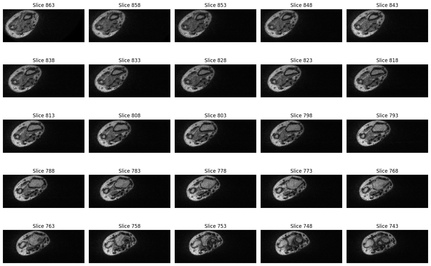
We will use the show_slices function to visualize the slices of the MRI data. Since we are interested in the transversal view of the hand, the function displays the images stored in the second dimension of the array.
from armscan_env.util.visualizations import show_slices

show_slices(
    data=mri_img,
    start=mri_img.shape[1] - 1,
    end=25,
    lap=5,
    extent=transversal_extent,
    cmap="gray",
)
plt.show()
Labelmaps dataset#
Next we will load the labelmaps data, which is also saved in the NIfTI format. The labelmaps have been created by manually segmenting the relevant tissues in the MRI data. The segmentation has been performed using ImFusion. The labelmaps are saved in the same coordinate system as the MRI data, and have the same size and spacing. Since they are saved in the same way as the MRI images, we can use the same functions to load and visualize them.
mri_1_label = sitk.ReadImage(config.get_single_labelmap_path(1))
mri_1_label_data = sitk.GetArrayFromImage(mri_1_label)
print(f"{mri_1_label_data.shape =}")
mri_1_label_data.shape =(61, 864, 606)
What is shown in the images, are the labeled tissues, hence bones, tendons, median nerve and ulnar artery.
show_slices(
    data=mri_1_label_data,
    start=mri_1_label_data.shape[1] - 1,
    end=25,
    lap=5,
    extent=transversal_extent,
)
plt.show()
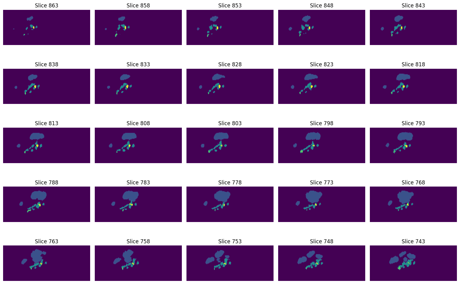
The labels are saved in the array as integers. Each voxel is assigned a label according to the following mapping:
0: background
1: bones
2: tendons
3: ulnar artery
4: median nerve
print("Max value in mri labeled data: ", np.max(mri_1_label_data))
print("Max value in mri data: ", np.max(mri_img))
Max value in mri labeled data:  4
Max value in mri data:  693