Show code cell content
import matplotlib.pyplot as plt
import numpy as np
import SimpleITK as sitk
from armscan_env.clustering import TissueClusters
from armscan_env.config import get_config
from armscan_env.envs.rewards import anatomy_based_rwd
from armscan_env.envs.state_action import ManipulatorAction
from armscan_env.util.visualizations import show_clusters
from armscan_env.volumes.volumes import ImageVolume
from celluloid import Camera
from IPython.core.display import HTML

config = get_config()
Arbitrary Slicing#
volume = sitk.ReadImage(config.get_single_labelmap_path(1))
volume_img = sitk.GetArrayFromImage(volume)

volume_size = volume.GetSize()
img_size = volume_img.shape
volume_origin = volume.GetOrigin()

physical_size = np.array(volume.GetSize()) * np.array(volume.GetSpacing())
print(f"{volume_size=}")
print(f"{img_size=}")
print(f"{physical_size=} mm")
transversal_extent = [0, physical_size[0], 0, physical_size[2]]
longitudinal_extent = [0, physical_size[1], 0, physical_size[2]]
frontal_extent = [0, physical_size[0], physical_size[1], 0]
volume_size=(606, 864, 61)
img_size=(61, 864, 606)
physical_size=array([150.0486095 , 213.93069077,  61.        ]) mm
Until now, we have only been able to visualize slices of the volume in the original orientation at which they were taken in the scan, and we defined a suboptimal view to visualize the carpal tunnel:
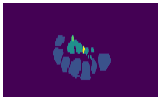
slice_num = 670
slice_ = volume_img[:, slice_num, :]
plt.imshow(slice_, aspect=6)
plt.axis("off")
plt.show()
However, it is necessary to view arbitrary planes of the volume, in order to be able to view the optimal plane, regardless of the orientation of the original scanned slices. In this notebook we are going to present a re-slicing algorithm to take arbitrary slices of the 3D volume. To do this, we can make use of the Euler3DTransform class from SimpleITK, which allows us to define a transformation matrix to reference our new plane, and Resaple, which samples the slice as a new image out of the original volume.
We need to define a Rotation matrix, a translation matrix, and the center of rotation, from which the transformation will be applied:
origin = np.array(volume.GetOrigin())
th_z = np.deg2rad(20)
th_x = np.deg2rad(0)
x_trans = 0
y_trans = 140

transform = sitk.Euler3DTransform()
transform.SetRotation(th_x, 0, th_z)
transform.SetTranslation((x_trans, y_trans, 0))
transform.SetCenter(origin)
We then need to define the resampling method, passing the volume we want to transform, the transformation matrix, and the interpolation method, which is set to nearest neighbor to preserve the integrity of the labels:
slice_volume = sitk.Resample(
    volume,
    transform,
    sitk.sitkNearestNeighbor,
    0.0,
    volume.GetPixelID(),
)
At this point we have created a reference frame for the plane we want to extract. We now need to sample the slice. Since the output is supposed to be a volume, we take a three dimensional slice, basically a stack of two images:
resampler = sitk.ResampleImageFilter()
resampler.SetReferenceImage(slice_volume)
resampler.SetSize((volume_size[0], 2, volume_size[2]))
resampler.SetInterpolator(sitk.sitkNearestNeighbor)
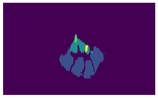
We can now finally view the slice, just by plotting one of the 2D resampled images we have extracted:
slice = resampler.Execute(slice_volume)[:, 0, :]
slice_img = sitk.GetArrayFromImage(slice)
print(f"{slice_img.shape=}")
plt.imshow(slice_img, aspect=6)
plt.axis("off")
plt.show()
slice_img.shape=(61, 606)
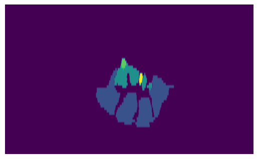
All of this is integrated in the ImageVolume class, which is a wrapper of the SimpleITK Image class, extended by the function get_volume_slice and by the attribute optimal_action, which permits to store the optimal rotation and translation parameters to view the standard plane of the carpal tunnel:
image_volume = ImageVolume(
    volume,
    optimal_action=ManipulatorAction(rotation=(19.3, 0), translation=(0, 140)),
)
sliced_volume = image_volume.get_volume_slice(
    action=image_volume.optimal_action,
    slice_shape=(image_volume.GetSize()[0], image_volume.GetSize()[2]),
)
slice_img = sitk.GetArrayFromImage(sliced_volume)
print(f"Slice value range: {np.min(slice_img)} - {np.max(slice_img)}")

print(slice_img.shape)
plt.imshow(slice_img, aspect=6)
plt.axis("off")
plt.show()
Slice value range: 0 - 4
(61, 606)
We can now perform clustering on the optimal image and see if it results in an optimal score, which is fulfilled under the threshold \(\delta=0.05\):
clusters = TissueClusters.from_labelmap_slice(slice_img.T)
show_clusters(clusters, slice_img.T)
reward = anatomy_based_rwd(clusters)
print(f"{reward=}")
plt.axis("off")
plt.show()
reward=-0.041666666666666664

Let’s now look at the beauty of this new slicing method by defining arbitrary transformations:
# Demonstration of arbitrary slicing
# y-translations
t = [160, 155, 150, 148, 146, 142, 140, 140, 115, 120, 125, 125, 130, 130, 135, 138, 140, 140, 140]
# z-rotations
z = [0, -5, 0, 0, 5, 15, 19.3, -10, 0, 0, 0, 5, -8, 8, 0, -10, -10, 10, 19.3]

# Create figure and subplots
fig, (ax1, ax2) = plt.subplots(1, 2, figsize=(8, 6))
camera = Camera(fig)
o = volume_origin


# Sample functions for demonstration
def linear_function(x: np.ndarray, m: float, b: float) -> np.ndarray:
    return m * x + b


for i in range(len(t)):
    # Subplot 1: Image with dashed line
    ax1.imshow(volume_img[40, :, :], extent=frontal_extent)
    x_dash = np.arange(physical_size[0])
    b = o[1] + t[i]
    y_dash = linear_function(x_dash, np.tan(np.deg2rad(z[i])), b)
    ax1.set_title(f"Section {i}")
    ax1.plot(x_dash, y_dash, linestyle="--", color="red")

    # Subplot 2: Function image
    sliced_volume = image_volume.get_volume_slice(
        slice_shape=(image_volume.GetSize()[0], image_volume.GetSize()[2]),
        action=ManipulatorAction(
            rotation=(z[i], 0),
            translation=(0, t[i]),
        ),
    )
    sliced_img = sitk.GetArrayFromImage(sliced_volume)
    ax2.set_title(f"Slice {i}")
    ax2.imshow(sliced_img, aspect=6)
    ax2.axis("off")
    camera.snap()
    plt.close()

animation = camera.animate()
HTML(animation.to_jshtml())
The Hard Way#
This can be done in a harder way, if you want to define the transformations yourself. This is actually the original way the function was developed, before coming across the SimpleITK Euler3DTransform class, and it might still be useful for integration with different software. The first step is to define an Euler transformation with the angles of rotation and the array of translation. This transformation matrix simulates the position and orientation of an ultrasound probe, scanning the arm to get a 2D image.
# Euler's transformation
# Rotation is defined by three rotations around z1, x2, z2 axis
th_z = np.deg2rad(20)
th_x = np.deg2rad(0)
x_trans = 0
y_trans = 140

# Translation vector
o = np.array(volume_origin)

# transformation simplified at th_y=0 since this rotation is never performed
eul_tr = np.array(
    [
        [np.cos(th_z), -np.sin(th_z) * np.cos(th_x), np.sin(th_z) * np.sin(th_x), o[0] + x_trans],
        [np.sin(th_z), np.cos(th_z) * np.cos(th_x), -np.cos(th_z) * np.sin(th_x), o[1] + y_trans],
        [0, np.sin(th_x), np.cos(th_x), o[2]],
        [0, 0, 0, 1],
    ],
)
After that, we define the coordinate system of the plane of the slice to take. The x and y coordinates are defined by the first two columns of the transformation matrix, and the normal vector of the plane is defined by the third column. The origin of the plane is defined by the last column of the transformation matrix, hence the translation from the image origin.
# Define plane's coordinate system
e1 = eul_tr[0][:3]  # x-coordinate of image plane
e2 = eul_tr[1][:3]  # y-coordinate of image plane
e3 = eul_tr[2][:3]  # normal vector of image plane
origin = eul_tr[:, -1:].flatten()[:3]  # origin of the image plane

print(f" {e1=},\n {e2=},\n {e3=},\n {origin=}")

# Direction for the resampler will be (e1, e2, e3) flattened
direction = np.stack([e1, e2, e3], axis=0).flatten()
print(f" {direction=}")
 e1=array([ 0.93969262, -0.34202014,  0.        ]),
 e2=array([ 0.34202014,  0.93969262, -0.        ]),
 e3=array([0., 0., 1.]),
 origin=array([-74.90050507,  33.1584549 , -30.        ])
 direction=array([ 0.93969262, -0.34202014,  0.        ,  0.34202014,  0.93969262,
       -0.        ,  0.        ,  0.        ,  1.        ])
he dimension of the new image will be set equal to the dimension of the images in the original transversal plane
h = volume_size[2]  # height of the image plane: original z size
w = volume_size[0]  # width of the image plane: original x size

print(f" {h=},\n {w=}")
 h=61,
 w=606
Finally, we use SimpleITK’s resampler to take the slice of the volume. We set the output direction, origin, and spacing to the ones defined by the plane. The size of the output image is defined by the width and height of the plane, and has a depth of 3 for visualization purposes when fed back into a volume renderer like ImFusion. The interpolator is set to nearest neighbor, since our label space is discrete.
# Use SimpleITK's resampler
resampler = sitk.ResampleImageFilter()
# Extract properties from the SimpleITK Image
spacing = volume.GetSpacing()

# use reference image
resampler.SetOutputDirection(direction.tolist())
resampler.SetOutputOrigin(origin.tolist())
resampler.SetOutputSpacing(spacing)
resampler.SetSize((w, 3, h))
resampler.SetInterpolator(sitk.sitkNearestNeighbor)
The output of the resampler is a 3D image, which we can convert to a numpy array and visualize. We can check that the value range corresponds to that of the labelmap.
sliced_volume = resampler.Execute(volume)
sliced_img = sitk.GetArrayFromImage(sliced_volume)

print(f"Slice value range: {np.min(sliced_img)} - {np.max(sliced_img)}")
print(f" {sliced_volume.GetSize()=},\n {volume_size=},\n {sliced_img.shape=},\n {img_size=}")
Slice value range: 0 - 4
 sliced_volume.GetSize()=(606, 3, 61),
 volume_size=(606, 864, 61),
 sliced_img.shape=(61, 3, 606),
 img_size=(61, 864, 606)
It is also possible to save the image has a .nii file for further visualization on a volume renderer. You can do this locally as follows:
output_path = os.path.join("../..", "data", "outputs", "sliced_volume.nii.gz")
sitk.WriteImage(sliced_volume, output_path)
We can now visualize the slice in a new orientation.
slice = sliced_img[:, 0, :]
plt.imshow(slice, aspect=6)
plt.axis("off")
plt.show()