%load_ext autoreload
%autoreload 2

import matplotlib.pyplot as plt
import numpy as np
import SimpleITK as sitk
from armscan_env import config
from armscan_env.clustering import TissueClusters
from armscan_env.envs.rewards import anatomy_based_rwd
from armscan_env.util.visualizations import show_clusters
from armscan_env.volumes.loading import (
    load_sitk_volumes,
    normalize_sitk_volumes_to_highest_spacing,
)

config = config.get_config()

Volumes Normalization

Let's load all the volumes in their original shape and in the normalized shape:

volumes = load_sitk_volumes(normalize=False)
normalized_volumes = normalize_sitk_volumes_to_highest_spacing(volumes)

Now you can set as volume any of the volumes (normalized or not). For the same volume, the array size will change, but the physical size will remain the same. The extent of the image will be set accordingly to the physical size.

volume = volumes[1]
volume_img = sitk.GetArrayFromImage(volume)
size = np.array(volume.GetSize()) * np.array(volume.GetSpacing())
print(f"{volume_img.shape=}")
print(f"{size=} mm")

volume_img.shape=(74, 272, 204)
size=array([105.00000286, 140.00000381,  74.        ]) mm

volume = normalized_volumes[1]
volume_img = sitk.GetArrayFromImage(volume)
size = np.array(volume.GetSize()) * np.array(volume.GetSpacing())
print(f"{volume_img.shape=}")
print(f"{size=} mm")
transversal_extent = (0, size[0], 0, size[2])
longitudinal_extent = (0, size[1], 0, size[2])
frontal_extent = (0, size[0], size[1], 0)

volume_img.shape=(74, 720, 540)
size=array([105.00000179, 140.00000238,  73.99992943]) mm

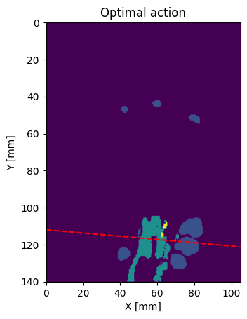
Let's visualize the optimal slice from the frontal view:

action = volume.optimal_action

spacing = volume.GetSpacing()
plt.imshow(volume_img[40, :, :], extent=frontal_extent)

o = volume.GetOrigin()
x_dash = np.arange(size[0])
b = action.translation[1]
y_dash = x_dash * np.tan(np.deg2rad(action.rotation[0])) + b
plt.plot(x_dash, y_dash, linestyle="--", color="red")
plt.title("Optimal action")
plt.ylabel("Y [mm]")
plt.xlabel("X [mm]")
plt.show()

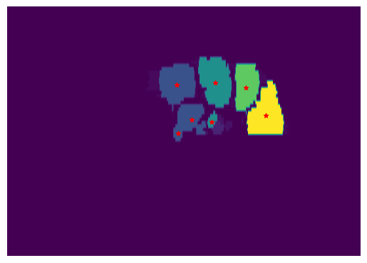
Now let's see if it corresponds to a optimal view of the carpal tunnel:

slice_shape = (volume.GetSize()[0], volume.GetSize()[2])
sliced_volume = volume.get_volume_slice(
    slice_shape=slice_shape,
    action=action,
)
sliced_img = sitk.GetArrayFromImage(sliced_volume)
cluster = TissueClusters.from_labelmap_slice(sliced_img.T)
show_clusters(cluster, sliced_img.T, extent=transversal_extent)
print(f"Slice value range: {np.min(sliced_img)} - {np.max(sliced_img)}")
plt.axis("off")
plt.show()

Slice value range: 0 - 4

The reward of the action depends on how well the clusters correspond to the anatomical description. It is difficult to tune the clustering so that it performs well in all volumes, so we set a threshold \(\delta\) to determine if the score is just good enough. The reward is then:

reward = anatomy_based_rwd(cluster)
print(reward)

-0.041666666666666664